Simple Moving Average (SMA)
I want to try and understand some existing algorithmic trading strategies. I suspect that the one trend we've found is probably a feature of a different strategy and its best on to reinvent the wheel. We're gonna start with a Simple Moving Average (SMA) strategy. The most basic form of this is taking an n-moving average line and if the stock price is above this line, it indicates the price is moving up. If the stock is below this line, it indicates that the price is moving down. I'm not going to hold any short positions.
We'll be using some code produced in a different post to collect and prepare the data.
| Close | Volume | Average Tone | Article Count | All Articles | |
|---|---|---|---|---|---|
| 2024-01-02 | 466.663971 | 123623700 | 0.1338 | 7402.0 | 113699.0 |
| 2024-01-03 | 462.852875 | 103585900 | -0.0392 | 8467.0 | 140100.0 |
| 2024-01-04 | 461.361969 | 84232200 | -0.0177 | 11418.0 | 171729.0 |
| 2024-01-05 | 461.993896 | 86060800 | 0.0540 | 9509.0 | 159932.0 |
| 2024-01-08 | 468.589294 | 74879100 | 0.1491 | 8584.0 | 145645.0 |
| ... | ... | ... | ... | ... | ... |
| 2024-12-20 | 591.150024 | 125716700 | 0.4267 | 11918.0 | 170707.0 |
| 2024-12-23 | 594.690002 | 57635800 | 0.3075 | 10892.0 | 169788.0 |
| 2024-12-24 | 601.299988 | 33160100 | 0.4874 | 8868.0 | 132293.0 |
| 2024-12-26 | 601.340027 | 41219100 | 0.4670 | 9350.0 | 142705.0 |
| 2024-12-27 | 595.010010 | 64969300 | 0.1646 | 10576.0 | 158638.0 |
250 rows × 5 columns
We will be using a SMA with and we will optimise later. The first thing to do is setup a strategy class. I've decided to avoid
from backtesting import Strategy, Backtest
from backtesting.lib import crossover
class SMA_1(Strategy):
n = 5
def init(self):
self.sma = self.I(SMA, self.data.Close, self.n, name = f"SMA ({self.n})")
def next(self):
if crossover(self.data.Close, self.sma):
self.buy()
if crossover(self.sma, self.data.Close):
self.position.close()
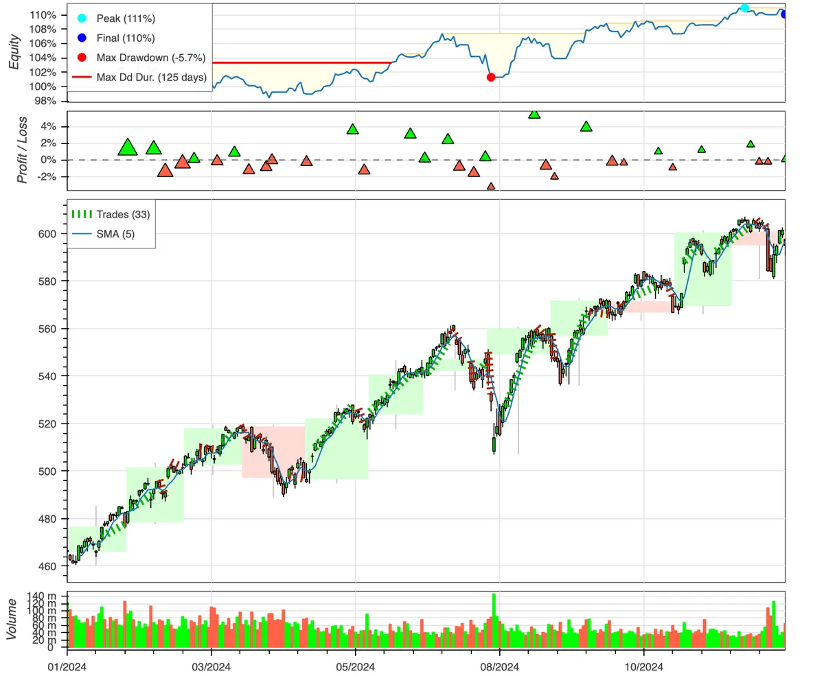
bt = Backtest(data, SMA_1, cash=10_000, commission=.002)
stats = bt.run()
bt.plot()
stats
Start                     2024-01-02 00:00:00
End                       2024-12-27 00:00:00
Duration                    360 days 00:00:00
Exposure Time [%]                        76.4
Equity Final [$]                  11009.11741
Equity Peak [$]                  11098.146572
Return [%]                          10.091174
Buy & Hold Return [%]               27.502881
Return (Ann.) [%]                   10.175879
Volatility (Ann.) [%]                 9.22326
Sharpe Ratio                         1.103284
Sortino Ratio                        1.741219
Calmar Ratio                         1.792502
Max. Drawdown [%]                   -5.676915
Avg. Drawdown [%]                   -1.350592
Max. Drawdown Duration      125 days 00:00:00
Avg. Drawdown Duration       23 days 00:00:00
# Trades                                   33
Win Rate [%]                        45.454545
Best Trade [%]                       5.398761
Worst Trade [%]                     -3.237501
Avg. Trade [%]                        0.28757
Max. Trade Duration          21 days 00:00:00
Avg. Trade Duration           7 days 00:00:00
Profit Factor                         1.62024
Expectancy [%]                       0.303059
SQN                                  0.969777
_strategy                               SMA_1
_equity_curve                             ...
_trades                       Size  EntryB...
dtype: object
Leading to a pretty terrible return compared to B&H. Looking at the plots, it shows that the equity is more or less following the actual market trend.
However, it might be the case that a more appropriate value for would result in a better return. For this, we can use optimisation. This usually takes quite a while to run but we're only considering 48 values.
stats, heatmap = bt.optimize(
    n = range(2, 50, 1),
    maximize='Equity Final [$]',
    max_tries=200,
    random_state=0,
    return_heatmap=True)
heatmap.sort_values().tail()
n
7    10989.254414
9    11008.870673
5    11009.117410
6    11093.484994
8    11155.974974
Name: Equity Final [$], dtype: float64
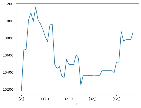
Therefore, is the best. Side note, here's a graph showing the "Equity Final [$]" against .
Performing the backtests again with this new value:
Start                     2024-01-02 00:00:00
End                       2024-12-27 00:00:00
Duration                    360 days 00:00:00
Exposure Time [%]                        74.8
Equity Final [$]                 11155.974974
Equity Peak [$]                  11299.692043
Return [%]                           11.55975
Buy & Hold Return [%]               27.502881
Return (Ann.) [%]                   11.657421
Volatility (Ann.) [%]                9.051886
Sharpe Ratio                         1.287844
Sortino Ratio                        2.112081
Calmar Ratio                         2.605327
Max. Drawdown [%]                   -4.474455
Avg. Drawdown [%]                   -1.192903
Max. Drawdown Duration       48 days 00:00:00
Avg. Drawdown Duration       16 days 00:00:00
# Trades                                   26
Win Rate [%]                        53.846154
Best Trade [%]                       4.676358
Worst Trade [%]                     -3.237501
Avg. Trade [%]                       0.431728
Max. Trade Duration          21 days 00:00:00
Avg. Trade Duration           9 days 00:00:00
Profit Factor                        2.016307
Expectancy [%]                       0.446811
SQN                                  1.243325
_strategy                               SMA_1
_equity_curve                             ...
_trades                       Size  EntryB...
dtype: object
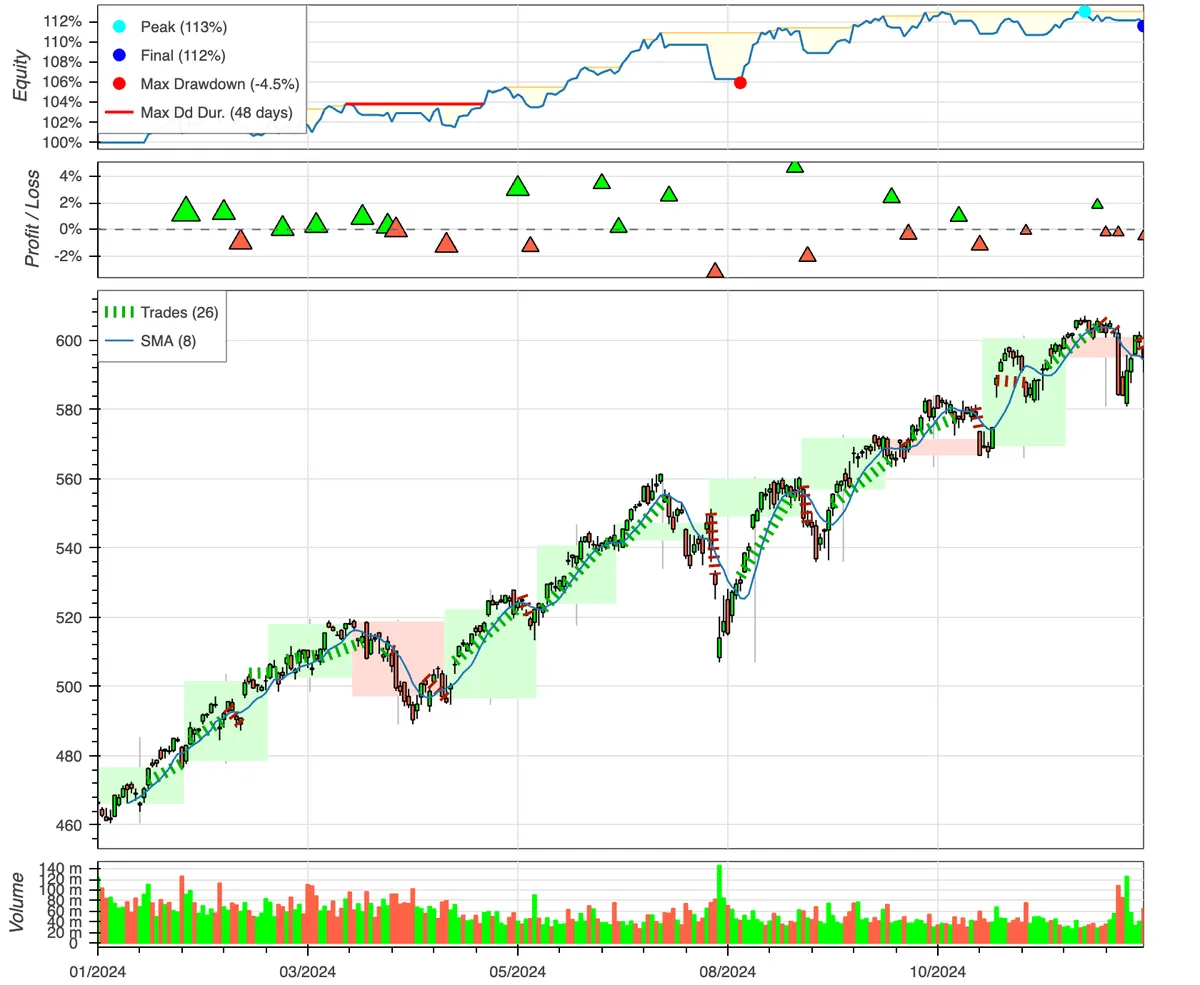
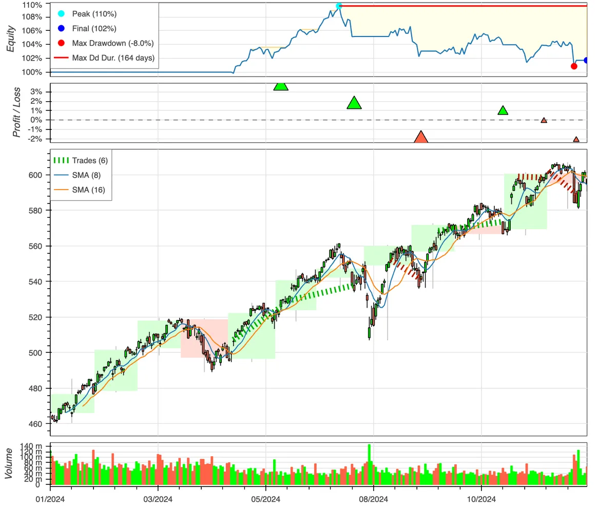
Still not great. Another strategy that involves SMA is to instead have two SMAs, a slow one and a fast one. If the fast moving one crosses over the slow moving one, we presume the stock is increasing. If the slow moving one crosses over the fast moving one, we presume the stock is decreasing.
The strategy I've used for this is below:
from backtesting import Strategy, Backtest
from backtesting.lib import crossover

class SMA_2(Strategy):
    n_fast = 7
    n_slow = 8
    def init(self):
       self.fast_sma = self.I(SMA, self.data.Close, self.n_fast, name = f"SMA ({self.n_fast})")
       self.slow_sma = self.I(SMA, self.data.Close, self.n_slow, name = f"SMA ({self.n_slow})")
    def next(self):
        if crossover(self.fast_sma, self.slow_sma):
          self.buy()

        elif crossover(self.slow_sma, self.fast_sma):
          self.position.close()


bt = Backtest(data, SMA_2, cash=10_000, commission=.002)
stats = bt.run()
bt.plot()
stats
Start                     2024-01-02 00:00:00
End                       2024-12-27 00:00:00
Duration                    360 days 00:00:00
Exposure Time [%]                        51.2
Equity Final [$]                 10171.149641
Equity Peak [$]                  10960.144571
Return [%]                           1.711496
Buy & Hold Return [%]               27.502881
Return (Ann.) [%]                    1.725306
Volatility (Ann.) [%]                7.548824
Sharpe Ratio                         0.228553
Sortino Ratio                        0.294205
Calmar Ratio                         0.216094
Max. Drawdown [%]                   -7.984061
Avg. Drawdown [%]                   -1.914544
Max. Drawdown Duration      164 days 00:00:00
Avg. Drawdown Duration       36 days 00:00:00
# Trades                                    6
Win Rate [%]                             50.0
Best Trade [%]                        3.62912
Worst Trade [%]                     -2.121228
Avg. Trade [%]                       0.306936
Max. Trade Duration          45 days 00:00:00
Avg. Trade Duration          29 days 00:00:00
Profit Factor                        1.464802
Expectancy [%]                       0.327355
SQN                                  0.315252
_strategy                               SMA_2
_equity_curve                             ...
_trades                      Size  EntryBa...
dtype: object
With the following optimisation:
stats, heatmap = bt.optimize(
    n_fast = range(2, 30, 1),
    n_slow = range(2, 30, 1),
    maximize='Equity Final [$]',
    constraint=lambda p: p.n_fast < p.n_slow,
    max_tries=200,
    random_state=0,
    return_heatmap=True)
heatmap.sort_values().tails()
n_fast  n_slow
12      28        11307.240472
4       5         11424.670926
3       8         11497.370173
        9         11618.003237
7       8         11757.419568
Name: Equity Final [$], dtype: float64
Not that great. The article made by backtesting.py used the second strategy on Google stock data and it looks like they got results that beat the market. I imagine it doesn't work on every stock though.